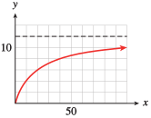
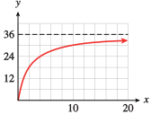
Francine is planning a 60-mile training flight through the desert on her cycle-plane, a pedal-driven aircraft. If there is no wind, she can pedal at an average speed of 15 miles per hour, so she can complete the flight in 4 hours.
If there is a headwind of \(x\) miles per hour, it will take Francine longer to fly 60 miles. Express the time it will take to complete the training flight as a function of \(x\text{.}\)
If there is a headwind of \(x\) miles per hour, Francine’s ground speed will be \(15 - x\) miles per hour. Using the fact that \(\text{time} = \dfrac{\text{distance}}{\text{rate}}\text{,}\) we find that the time needed for the flight will be
\begin{equation*}
t = f (x) = \frac{60}{15 - x}
\end{equation*}
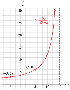
Francine’s effective speed is only \(10\) miles per hour, and it will take her \(6\) hours to fly the \(60\) miles. The table shows that as the speed of the headwind increases, the time required for the flight increases also.
to verify the graph. In particular, the point \((0, 4)\) lies on the graph. This point tells us that if there is no wind, Francine can fly \(60\) miles in \(4\) hours, as we calculated earlier.
The graph is increasing, as indicated by the table of values. In fact, as the speed of the wind gets close to \(15\) miles per hour, Francine’s flying time becomes extremely large. In theory, if the wind speed were exactly \(15\) miles per hour, Francine would never complete her flight. On the graph, the time becomes infinite at \(x = 15\text{.}\)
What about negative values for \(x\text{?}\) If we interpret a negative headwind as a tailwind, Francine’s flying time should decrease for negative \(x\)-values. For example, if \(x = -5\text{,}\) there is a tailwind of \(5\) miles per hour, so Francine’s effective speed is \(20\) miles per hour, and she can complete the flight in \(3\) hours. As the tailwind gets stronger (that is, as we move farther to the left in the \(x\)-direction), Francine’s flying time continues to decrease, and the graph approaches the \(x\)-axis.
The vertical dashed line at \(x=15\) on the graph of \(t=\dfrac{60}{15-x}\) is a vertical asymptote for the graph. We first encountered asymptotes in Section 2.2 when we studied the graph of \(y=\dfrac{1}{x}\text{.}\) Locating the vertical asymptotes of a rational function is an important part of determining the shape of the graph.
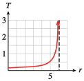
Queueing theory is used to predict your waiting time in a line, or queue. For example, suppose the attendant at a toll booth can process \(6\) vehicles per minute. The average total time spent by a motorist negotiating the toll booth depends on the rate, \(r\text{,}\) at which vehicles arrive, according to the formula
EarthCare decides to sell T-shirts to raise money. The company makes an initial investment of $100 to pay for the design of the T-shirt and to set up the printing process. After that, the T-shirts cost $5 each for labor and materials.
Express the average cost per T-shirt as a function of the number of T-shirts EarthCare produces.
If EarthCare produces \(x\) T-shirts, the total costs will be \(100 + 5x\) dollars. To find the average cost per T-shirt, we divide the total cost by the number of T-shirts produced, to get
\begin{equation*}
C = g(x) = \frac{100 + 5x}{x}
\end{equation*}
If EarthCare makes only one T-shirt, its cost is $105. But if more than one T-shirt is made, the cost of the original $100 investment is distributed among them. For example, the average cost per T-shirt for \(\alert{2}\) T-shirts is
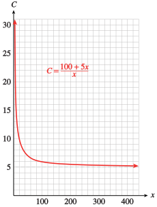
to verify the graph. Use the Trace to locate on the graph several points from the table of values. For example, the point \((5, 25)\) indicates that if EarthCare makes \(5\) T-shirts, the cost per shirt is $\(25\text{.}\)
The graph shows that as the number of T-shirts increases, the average cost per shirt continues to decrease, but not as rapidly as at first. Eventually the average cost levels off and approaches $5 per T-shirt. For example, if EarthCare produces \(\alert{400}\) T-shirts, the average cost per shirt is
The horizontal line \(C = 5\) on the graph of \(C = \displaystyle{\frac{100 + 5x}{x}}\) is a horizontal asymptote. As \(x\) increases, the graph approaches the line \(C = 5\) but never actually meets it. The average price per T-shirt will always be slightly more than $5. Horizontal asymptotes are also important in sketching the graphs of rational functions.
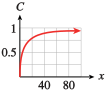
Delbert prepares a 20% glucose solution by mixing 2 mL of glucose with 8 mL of water. If he adds \(x\) ml of glucose to the solution, its concentration is given by
Most applications of rational functions have restricted domains, that is, they make sense for only a subset of the real numbers on the \(x\)-axis. Consequently, only a portion of the graph is useful for analyzing the application. However, a knowledge of the general shape and properties of the whole graph can be very helpful in understanding a rational function.
Because we cannot divide by zero, a rational function \(~f(x) = \displaystyle{\frac{P(x)}{Q(x)}}~\) is undefined for any value \(x = a\) where \(Q(a) = 0\text{.}\) These \(x\)-values are not in the domain of the function.
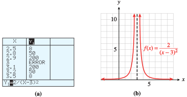
The domain of \(f\) is the set of all real numbers except \(3\text{,}\) because the denominator, \((x - 3)^2\text{,}\) equals \(0\) when \(x = 3\text{.}\)
The domain of \(k\) is the set of all real numbers except \(3\) and \(-3\text{,}\) because \(x^2 - 9\) equals \(0\) when \(x = 3\) or \(x = -3\text{.}\)
We only need to exclude the zeros of the denominator from the domain of a rational function. We do not exclude the zeros of the numerator. In fact, the zeros of the numerator include the zeros of the rational function itself, because a fraction is equal to \(0\) when its numerator is \(0\) but its denominator is not \(0\text{.}\)
As we saw in Section 7.2, a polynomial function is defined for all values of \(x\text{,}\) and its graph is a smooth curve without any breaks or holes. The graph of a rational function, on the other hand, will have breaks or holes at those \(x\)-values where it is undefined.
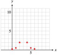
This function is undefined for \(x = 3\text{,}\) so there is no point on the graph with \(x\)-coordinate \(3\text{.}\) However, we can make a table of values for other values of \(x\text{.}\) Plotting the ordered pairs in the table results in the points shown below.
Next, we make a table showing \(x\)-values close to \(3\text{,}\) as shown below. As we choose \(x\)-values closer and closer to \(3\text{,}\)\((x - 3)^2\) gets closer to \(0\text{,}\) so the fraction \(\dfrac{2}{(x-3)^2}\) gets very large. This means that the graph approaches, but never touches, the vertical line \(x=3\text{.}\) In other words, the graph has a vertical asymptote at \(x=3\text{.}\) We indicate the vertical asymptote by a dashed line, as shown in the figure.
If \(Q(a) = 0\) but \(P(a) \ne 0\text{,}\) then the graph of the rational function \(f(x) = \displaystyle{\frac{P(x)}{Q(x)}}\) has a vertical asymptote at \(x=a\text{.}\)
If \(P(a)\) and \(Q(a)\) are both zero, then the graph of the rational function \(\displaystyle{\frac{P(x)}{Q(x)}}\) may have a hole at \(x=a\) rather than an asymptote. (This possibility is considered in the homework exercises.)
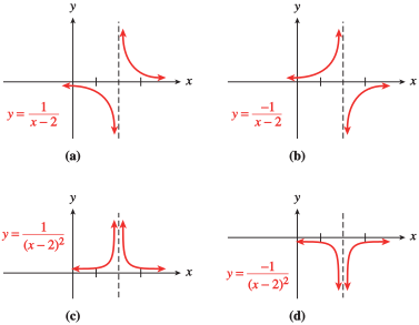
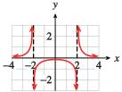
Near a vertical asymptote, the graph of a rational function has one of the four characteristic shapes, illustrated below. Locating the vertical asymptotes can help us make a quick sketch of a rational function.
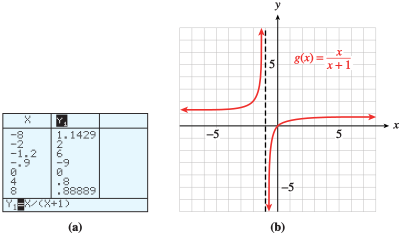
The denominator, \(x+1\text{,}\) equals zero when \(x = -1\text{.}\) Because the numerator does not equal zero when \(x = -1\text{,}\) there is a vertical asymptote at \(x = -1\text{.}\) The asymptote separates the graph into two pieces.
We can use the Table feature of a calculator to evaluate \(g(x)\) for several values of \(x\) on either side of the asymptote, as shown in figure (a). We plot the points found in this way; then connect the points on either side of the asymptote to obtain the graph shown in figure (b).
Look again at the graph of \(g(x) = \displaystyle{\frac{x}{x + 1}}\) in Example 7.86. As \(\abs{x}\) gets large—that is, as we move away from the origin along the \(x\)-axis in either direction—the corresponding \(y\)-values get closer and closer to \(1\text{.}\) The graph approaches, but never coincides with, the line \(y=1\text{.}\) We say that the graph has a horizontal asymptote at \(y=1\text{.}\)
When does a rational function \(f(x) = \displaystyle{\frac{P(x)}{Q(x)}}\) have a horizontal asymptote? It depends on the degrees of the two polynomials \(P(x)\) and \(Q(x)\text{.}\) The degree of the numerator of \(g(x)= \displaystyle{\frac{x}{x + 1}}\) is equal to the degree of the denominator. In other words, the highest power of \(x\) in the numerator (1, in this case) is the same as the highest power in the denominator.
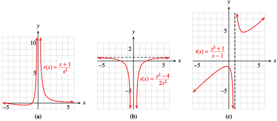
The graph of \(r(x) = \displaystyle{\frac{x + 1}{x^2}}\) in figure (a) has a horizontal asymptote at \(y = 0\text{,}\) the \(x\)-axis, because the degree of the denominator is larger than the degree of the numerator. Higher powers of \(x\) grow much more rapidly than smaller powers. Thus, for large values of \(\abs{x}\text{,}\) the denominator is much larger in absolute value than the numerator of \(r(x)\text{,}\) so the function values approach \(0\text{.}\)
The graph of \(s(x) = \displaystyle{\frac{x^2 - 4}{2x^2}}\) in figure (b) has a horizontal asymptote at \(y = \dfrac{1}{2}\text{,}\) because the numerator and denominator of the fraction have the same degree. For large values of \(\abs{x}\text{,}\) the terms of lower degree are negligible compared to the squared terms. As \(x\) increases, \(s(x)\) is approximately equal to \(\dfrac{x^2}{2x^2}\text{,}\) or \(\dfrac{1}{2}\text{.}\) Thus, the function values approach a constant value of \(\dfrac{1}{2}\text{.}\)
The graph of \(t(x) = \displaystyle{\frac{x^2 + 1}{x - 1}}\) in figure (c) does not have a horizontal asymptote, because the degree of the numerator is larger than the degree of the denominator. As \(\abs{x}\) increases, \(x^2 + 1\) grows much faster than \(x - 1\text{,}\) so their ratio does not approach a constant value. The function values increase without bound.
Suppose \(f(x) = \displaystyle{\frac{P(x)}{Q(x)}}\) is a rational function, where the degree of \(P(x)\) is \(m\) and the degree of \(Q(x)\) is \(n\text{.}\)
If \(m\lt n\text{,}\) the graph of \(f\) has a horizontal asymptote at \(y=0\text{.}\)
If \(m = n\text{,}\) the graph of \(f\) has a horizontal asymptote at \(y = \dfrac{a}{b}\text{,}\) where \(a\) is the lead coefficient of \(P(x)\) and \(b\) is the lead coefficient of \(Q(x)\text{.}\)
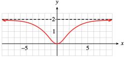
The numerator and denominator of the fraction are both second-degree polynomials, so the graph does have a horizontal asymptote. The lead coefficients of \(P(x)\) and \(Q(x)\) are \(2\) and \(1\text{,}\) respectively, so the horizontal asymptote is \(y = \dfrac{2}{1}\text{,}\) or \(y=2\text{.}\)
The \(y\)-intercept of the graph is the point \((0, 0)\text{.}\) We can plot several points by evaluating the function at convenient \(x\)-values, and use the asymptote to help us sketch the graph, as shown below.
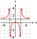
Locate the horizontal and vertical asymptotes and sketch the graph of \(~k(x) = \displaystyle{\frac{x^2 - 1}{x^2 - 9}}\text{.}\) Label the \(x\)- and \(y\)-intercepts with their coordinates.
It is often useful to simplify the formula for a rational function before using it. (See Algebra Skills Refresher Section A.9 to review operations on algebraic fractions.)
When estimating their travel time, pilots must take into account the prevailing winds. A tailwind adds to the plane’s ground speed, while a headwind decreases the ground speed. Skyhigh Airlines is setting up a shuttle service from Dallas to Phoenix, a distance of \(800\) miles.
Suppose there is a prevailing wind of \(30\) miles per hour blowing from the west. Write expressions for the flying time from Dallas to Phoenix and from Phoenix to Dallas.
Write an expression for the round-trip flying time, excluding stops, with a \(30\)-mile-per-hour wind from the west, as a function of the plane’s speed. Simplify your expression.
Recall that \(\text{time} = \dfrac{\text{distance}}{\text{rate}}\text{.}\) If we let \(r\) represent the speed of the plane in still air, then the time required for a one-way trip is
On the trip from Dallas to Phoenix, the plane encounters a headwind of \(30\) miles per hour, so its actual ground speed is \(r-30\text{.}\) On the return trip, the plane enjoys a tailwind of \(30\) miles per hour, so its actual ground speed is \(r+30\text{.}\) Therefore, the flying times are
\begin{equation*}
\text{Dallas to Phoenix:}\hphantom{blank}\frac{800}{r-30}
\end{equation*}
and
\begin{equation*}
\text{Phoenix to Dallas:}\hphantom{blank}\frac{800}{r+30}
\end{equation*}
Navid took his outboard motorboat 20 miles upstream to a fishing site, returning downstream later that day. His boat travels 10 miles per hour in still water. Write an expression for the time Navid spent traveling, as a function of the speed of the current. Let \(x\) represent the speed of the current in miles per hour.
A rational function \(f (x) = \dfrac{P(x)}{Q(x)}\) is undefined for any value \(x=1\) where \(Q(a) = 0\text{.}\) These \(x\)-values are not in the domain of the function.
If \(Q(a) = 0\) but \(P(a) \ne 0\text{,}\) then the graph of the rational function \(f(x) = \displaystyle{\frac{P(x)}{Q(x)}}\) has a vertical asymptote at \(x=a\text{.}\)
Suppose \(f(x) = \displaystyle{\frac{P(x)}{Q(x)}}\) is a rational function, where the degree of \(P(x)\) is \(m\) and the degree of \(Q(x)\) is \(n\text{.}\)
If \(m\lt n\text{,}\) the graph of \(f\) has a horizontal asymptote at \(y=0\text{.}\)
If \(m = n\text{,}\) the graph of \(f\) has a horizontal asymptote at \(y = \dfrac{a}{b}\text{,}\) where \(a\) is the lead coefficient of \(P(x)\) and \(b\) is the lead coefficient of \(Q(x)\text{.}\)
The eider duck, one of the world’s fastest flying birds, can exceed an airspeed of \(65\) miles per hour. A flock of eider ducks is migrating south at an average airspeed of \(50\) miles per hour against a moderate headwind. Their next feeding grounds are \(150\) miles away.
Express the ducks’ travel time, \(t\text{,}\) as a function of the windspeed, \(v\text{.}\)
Use the table to choose an appropriate window and graph your function \(t(v) \text{.}\) Give the equations of any horizontal or vertical asymptotes. What does the vertical asymptote signify in the context of the problem?
The fastest fish in the sea may be the bluefin tuna, which has been clocked at \(43\) miles per hour in short sprints. A school of tuna is migrating a distance of \(200\) miles at an average speed of \(36\) miles per hour in still water, but they have run into a current flowing against their direction of travel.
Express the tuna’s travel time, \(t\text{,}\) as a function of the current speed, \(v\text{.}\)
Use the table to choose an appropriate window and graph your function \(t(v) \text{.}\) Give the equations of any horizontal or vertical asymptotes. What does the vertical asymptote signify in the context of the problem?
Graph the function \(C\text{.}\) (Use \(\text{Xmin} = 6\text{,}\)\(\text{Xmax}= 100\text{,}\) and appropriate values of \(\text{Ymin}\) and \(\text{Ymax}.\)) What percentage of the population can be immunized if the city is able to spend $\(108,000\text{?}\)
Graph the function \(C\text{.}\) (Use \(\text{Xmin} = 6\text{,}\)\(\text{Xmax}= 100\text{,}\) and appropriate values of \(\text{Ymin}\) and \(\text{Ymax}.\)) What percentage of the ore can be extracted if \($540,000\) can be spent on the extraction?
Using the formula for \(D(p)\text{,}\) write an expression \(R(p)\) that approximates the total daily revenue as a function of the price, \(p\text{.}\)
Graph the revenue function \(R(p)\) in the same window with \(D(p) \text{.}\) Estimate the maximum possible revenue. Does the maximum for \(D(p)\) occur at the same value of \(p\) as the maximum for \(R(p)\text{?}\)
A computer store sells approximately \(300\) of its most popular model per year. The manager would like to minimize her annual inventory cost by ordering the optimal number of computers, \(x\text{,}\) at regular intervals. If she orders \(x\) computers in each shipment, the cost of storage will be \(6x\) dollars, and the cost of reordering will be \(\dfrac{300}{x} (15x + 10)\) dollars. The inventory cost is the sum of the storage cost and the reordering cost.
Use the distributive law to simplify the expression for the reordering cost. Then express the inventory cost, \(C\text{,}\) as a function of \(x\text{.}\)
A chain of electronics stores sells approximately \(500\) cellphones every year. The owner would like to minimize his annual inventory cost by ordering the optimal number of phones, \(x\text{,}\) at regular intervals. The cost of storing the phones will then be \(2x\) dollars, and the cost of reordering will be \(\dfrac{500}{x}(4x + 10) \text{.}\) The total annual inventory cost is the sum of the storage cost and the reordering cost.
Use the distributive law to simplify the expression for the reordering cost. Then express the inventory cost, \(C\text{,}\) as a function of \(x\text{.}\)
Francine wants to make a rectangular box. In order to simplify construction and keep her costs down, she plans for the box to have a square base and a total surface area of \(96\) square centimeters. She would like to know the largest volume that such a box can have.
If the square base has length \(x\) centimeters, show that the height of the box is \(h = \dfrac{24}{x}- \dfrac{x}{2}\) centimeters. (Hint: The surface area of the box is the sum of the areas of the six sides of the box.)
Graph your expression for volume \(V(x)\) in an appropriate window. Approximate the maximum possible volume for a box of surface area \(96\) square centimeters.
Graph the height, \(h(x)\text{,}\) in the same window with \(V(x)\text{.}\) What is the height of the box with greatest volume? (Find the height directly from your graph and verify by using the formula given for \(h(x)\text{.}\))
Delbert wants to make a box with a square base and a volume of \(64\) cubic centimeters. He would like to know the smallest surface area that such a box can have.
If the square base has length \(x\) centimeters, show that the height of the box is \(h = \dfrac{64}{x^2}\) centimeters.
Write an expression for the surface area, \(S\text{,}\) of the box as a function of the length, \(x\text{,}\) of its base. (Hint: The surface area of the box is the sum of the areas of the six sides of the box.)
Graph the height, \(h(x)\text{,}\) in the same window with \(S(x)\text{.}\) What is the height of the box with smallest surface area? (Find the height directly from your graph and verify by using the formula given for \(h(x)\text{.}\))
A train whistle sounds higher when the train is approaching you than when it is moving away from you. This phenomenon is known as the Doppler effect. If the actual pitch of the whistle is \(440\) hertz (this is the A note below middle C), then the note you hear will have the pitch
where the velocity, \(v\text{,}\) in meters per second is positive as the train approaches and is negative when the train is moving away. (The number \(332\) that appears in this expression is the speed of sound in meters per second.)
Complete the table of values showing the pitch of the whistle at various train velocities.
Graph the function \(P\text{.}\) (Use the window \({\text{Xmin}} = -94\text{,}\)\({\text{Xmax}} = 94\text{,}\) and appropriate values of \(\text{Ymin}\) and \(\text{Ymax}.\))
What is the velocity of the train if the note you hear has a pitch of \(415\) hertz (corresponding to the note A-flat)? A pitch of \(553.\overline{3}\) hertz (C-sharp)?
where \(v\) is the speed (in meters per second) at which the projectile was launched. (The radius of the Earth is \(6.4\times 10^6\) meters, and the constant \(19.6\) is related to the Earth’s gravitational constant.)
Complete the table of values showing the maximum altitude for various launch velocities.
Graph the function \(h\text{.}\) (Use the window \({\text{Xmin}} = 0\text{,}\)\({{\text{Xmax}}} = 940\text{,}\) and appropriate values of \(\text{Ymin}\) and \(\text{Ymax}.\))
River Queen Tours offers a \(50\)-mile round-trip excursion on the Mississippi River on a paddle wheel boat. The current in the Mississippi is \(8\) miles per hour.
Express the time required for the downstream journey as a function of the speed of the paddle wheel boat in still water.
A rowing team can maintain a speed of \(15\) miles per hour in still water. The team’s daily training session includes a \(5\)-mile run up the Red Cedar River and the return downstream.
Express the team’s time on the upstream leg as a function of the speed of the current.
Two pilots for the Flying Express parcel service receive packages simultaneously. Orville leaves Boston for Chicago at the same time Wilbur leaves Chicago for Boston. Each selects an airspeed of \(400\) miles per hour for the \(900\)-mile trip. The prevailing winds blow from east to west.
Express Orville’s flying time as a function of the windspeed.
On New Year’s Day, a blimp leaves its berth in Carson, California, and heads north for the Rose Bowl, \(23\) miles away. There is a breeze from the north at \(6\) miles per hour.
Express the time required for the trip as a function of the blimp’s airspeed.
where \(f\) stands for the focal length, \(p\) is the distance from the object viewed to the lens, and \(q\) is the distance from the image to the lens. Suppose you estimate that the distance from your cat (the object viewed) to your camera lens is \(60\) inches greater than the distance from the lens to the film inside the camera, where the image forms.
Express \(1/f\) as a single fraction in terms of \(q\text{.}\)
If two resistors, \(R_1\) and \(R_2\text{,}\) in an electrical circuit are connected in parallel, the total resistance \(R\) in the circuit is given by
Suppose that the second resistor, \(R_2\text{,}\) is \(10\) ohms greater than the first. Express \(1/R\) as a single fraction in terms of \(R_1\text{.}\)
The Michaelis-Menten equation is the rate equation for chemical reactions catalyzed by enzymes. The speed of the reaction \(v\) is a function of the initial concentration of the reactant \(s\) and is given by
\begin{equation*}
v = f(s) = \frac{Vs}{s+K}
\end{equation*}
where \(V\) is the maximum possible reaction rate and \(K\) is called the Michaelis constant. (Source: Holme and Peck, 1993)
What value does \(v\) approach as \(s\) increases?
Refer to the Michaelis-Menten equation in Problem 49. Solve for \(\dfrac{1}{v} \text{,}\) then write your new equation in the form \(\dfrac{1}{v}= a\cdot \dfrac{1}{s}+b \text{.}\) Express \(a\) and \(b\) in terms of \(V\) and \(K\text{.}\)
Refer to the Michaelis-Menten equation in Problem 49. Write an equation for \(\dfrac{s}{v} \) in the form \(\dfrac{s}{v}= cs+d \text{.}\) Express \(c\) and \(d\) in terms of \(V\) and \(K\text{.}\)
Graph the function. (Hint: The graph of the original function is identical to the graph of the function in part (b) except that certain points are excluded from the domain.) Indicate a hole in the graph by an open circle.