Subsection Logarithms and Exponents
Before we look at logarithmic functions, let’s quickly review exponents and logs. For a particular base, let’s say 5, taking a logarithm is the opposite operation for raising to a power. For example, if we raise base 5 to a power of \(\alert{2}\text{,}\) we get
\begin{equation*}
5^\alert{2} = 25 ~~~~ \text{and thus} ~~~~ \log_5 {(25)} = \alert{2}
\end{equation*}
We can say that a logarithm is actually an exponent. Asking for the log base 5 of 25 is asking "what power of 5, or what exponent on base 5 will give me 25?"
Example 5.30.
Write each logarithmic equation as an equivalent exponential equation.
\(\displaystyle \log_3 {(81)} = 4\)
\(\displaystyle \log_b {(32)} = 5\)
Solution.
The logarithm asks "To what power must I raise 3 to get 81?" The base is 3 and the logarithm (or exponent) is 4, so \(3^4 = 81\text{.}\)
The logarithm asks "To what power must I raise \(b\) to get 32?" The base is \(b\) and the logarithm (or exponent) is 5, so \(b^5 = 32\text{.}\)
For a more thorough review of logarithms you can refer to
Section 4.3.1.
Checkpoint 5.31. QuickCheck 1.
Which of these could you use to estimate the value of \(\log_5 {(378)}\) ?
Find multiples of 5.
Find the fifth root of 378.
Find powers of 5.
Divide 378 by 5.
Now we’ll consider functions defined in terms of logarithms, or logarithmic functions. For example,
\begin{equation*}
f(x)=\log_2 {(x)}
\end{equation*}
is a logarithmic function. In order to understand logarithmic functions better, we first investigate how they are related to more familiar functions, the exponential functions.
Subsection Inverse of the Exponential Function
Inverse functions are really a generalization of inverse operations. For example, raising to the \(n\)th power and taking \(n\)th roots are inverse operations. In fact, we use the following rule to define cube roots:
\begin{equation*}
\sqrt[3]{b} = a ~~~~\text{ if and only if }~~~~ a^3 = b
\end{equation*}
Compare this rule to the definition of inverse functions from
Section 5.1.
Inverse Functions.
Suppose \(g\) is the inverse function for \(f\text{.}\) Then
\begin{equation*}
g(b) = a~~~~~ \text{ if and only if }~~~~~f(a) = b
\end{equation*}
In this case, \(~g(x) = \sqrt[3]{x}~\) and \(~f(x) = x^3~\text{,}\) and the equations above tell us that the two functions \(~f(x) = x^3~\) and \(~g(x) = \sqrt[3]{x}~\) are inverse functions.
In
Chapter 4, we saw that a similar rule relates the operations of raising a base
\(b\) to a power and taking a base
\(b\) logarithm, because they are inverse operations.
Conversion Formulas for Logarithms.
For any base \(b \gt 0, b\ne 1\text{,}\)
\begin{equation*}
\blert{\log_{b}{x} = y} ~~~~\text{ if and only if }~~~~ \blert{b^y = x}
\end{equation*}
We can now define the logarithmic function, \(~g(x) = \log_{b}{x}\text{,}\) that takes the log base \(b\) of its input values. The conversion formulas tell us that the log function, \(~g(x) = \log_{b}{x}\text{,}\) is the inverse of the exponential function, \(~f(x) = b^x\text{.}\)
Logarithmic Function.
The logarithmic function base \(b\text{,}\)
\begin{equation*}
~g(x) = \log_b x~\text{,}
\end{equation*}
is the inverse of the exponential function of the same base, \(f(x) = b^x\text{.}\)
Subsection Graphs of Logarithmic Functions
What does the graph of a log function look like? We can use exponential functions to help us.
We can obtain a table of values for \(~g(x) = \log_2 x~\) by making a table for \(~f(x) = 2^x~\) and then interchanging the columns, as shown in the tables below. You can see that the graphs of \(~f(x) = 2^x~\) and \(~g(x) = \log_2 x\text{,}\) shown in the figure, are symmetric about the line \(y = x\text{.}\)
| \(x\) |
\(f(x)=2^x\) |
| \(-2\) |
\(\dfrac{1}{4}\) |
| \(-1\) |
\(\dfrac{1}{2}\) |
| \(0\) |
\(1\) |
| \(1\) |
\(2\) |
| \(2\) |
\(4\) |
| \(x\) |
\(g(x)=\log_{2}{x}\) |
| \(\dfrac{1}{4}\) |
\(-2\) |
| \(\dfrac{1}{2}\) |
\(-1\) |
| \(1\) |
\(0\) |
| \(2\) |
\(1\) |
| \(4\) |
\(2\) |
The same procedure works for graphing log functions with any base: If we want to find values for the function \(~y=\log_b x\text{,}\) we can find the values for the exponential function \(~y=b^x\text{,}\) and then interchange the \(x\) and \(y\) values in each ordered pair.
Example 5.32.
Graph the function \(~f(x)=10^x~\) and its inverse \(~g(x)=\log_{10}{x}~\) on the same axes.
Solution.
We start by making a table of values for the function \(f(x)=10^x\text{.}\) We can make a table of values for the inverse function, \(~g(x) = \log_{10}{x}~\text{,}\) by interchanging the components of each ordered pair in the table for \(f\text{.}\)
| \(x\) |
\(f(x)\) |
| \(-2\) |
\(0.01\) |
| \(-1\) |
\(0.1\) |
| \(0\) |
\(1\) |
| \(1\) |
\(10\) |
| \(2\) |
\(100\) |
| \(x\) |
\(g(x)\) |
| \(0.01\) |
\(-2\) |
| \(0.1\) |
\(-1\) |
| \(1\) |
\(0\) |
| \(10\) |
\(1\) |
| \(100\) |
\(2\) |
We plot each set of points and connect them with smooth curves to obtain the graphs shown above.
Checkpoint 5.33. Practice 1.
Complete the table of values and graph the function \(~h(x) = \log_4 x\text{.}\)
| \(x\) |
\(~\dfrac{1}{4}~\) |
\(~1~\) |
\(~2~\) |
\(~4~\) |
\(~16~\) |
| \(\log_4 x\) |
\(\hphantom{000}\) |
\(\hphantom{000}\) |
\(\hphantom{000}\) |
\(\hphantom{000}\) |
\(\hphantom{000}\) |
Solution.
| \(x\) |
\(~\dfrac{1}{4}~\) |
\(~1~\) |
\(~2~\) |
\(~4~\) |
\(~16~\) |
| \(\log_4 x\) |
\(-1\) |
\(0\) |
\(\dfrac{1}{2}\) |
\(1\) |
\(2\) |
Checkpoint 5.34. QuickCheck 2.
What is the \(y\)-intercept of the graph of \(~y=\log_5 x\) ?
\(\displaystyle (0,1)\)
\(\displaystyle (1,0)\)
\(\displaystyle (0,5)\)
There is none.
You can also see that while an exponential growth function increases very rapidly for positive input values, its inverse, the logarithmic function, grows extremely slowly.
In addition, the logarithmic function \(~y = \log_b x~\) has the following properties.
Logarithmic Functions \(~y = \log_b x\).
Domain: all positive real numbers
Range: all real numbers
\(x\)-intercept: \((1, 0)\)
\(y\)-intercept: none
Vertical asymptote at \(x = 0\)
The graphs of \(~y = \log_b x~\) and \(~y = b^x~\) are symmetric about the line \(y = x\text{.}\)
Checkpoint 5.36. QuickCheck 3.
The domain of the function \(~g(x)=\log_3 x\) is
all real numbers.
all multiples of 3.
all non-negative numbers.
all positive numbers.
Checkpoint 5.37. Pause and Reflect.
Why does the function \(~f(x)=\log x~\) grow so slowly?
Subsection Modeling with Logarithmic Functions
We can use the LOG key on a calculator to evaluate the function \(~f(x) = \log_{10}{x}\text{.}\)
Example 5.38.
Let \(~f(x) = \log_{10}{x}\text{.}\) Evaluate the following expressions.
\(\displaystyle f(35)\)
\(\displaystyle f(-8)\)
\(\displaystyle 2 f(16) + 1\)
Solution.
\(\displaystyle f(35) = \log_{10}{35}\approx 1.544\)
Because \(-8\) is not in the domain of \(f\text{,}\) \(f(-8)\text{,}\) or \(\log_{10}{(-8)}\text{,}\) is undefined.
\(\displaystyle 2 f(16) + 1 = 2(\log_{10}{16}) + 1\approx2(1.204) + 1 = 3.408\)
Checkpoint 5.39. QuickCheck 4.
Which statement is true?
The log of a number is never negative.
We cannot take the log of a negative number.
The log of a fraction is called a common log.
The log of 0 is 1.
Checkpoint 5.40. Practice 2.
The formula
\begin{equation*}
T = \dfrac{\log 2 \cdot t_i}{3 \log(D_f /D_0)}
\end{equation*}
is used by X-ray technicians to calculate the doubling time of a malignant tumor. \(D_0\) is the diameter of the tumor when first detected, \(D_f\) is its diameter at the next reading, and \(t_i\) is the time interval between readings, in days.
Calculate the doubling time of the following tumor: its diameter when first detected was 1 cm, and 7 days later its diameter was 1.05 cm.
Solution.
\(T= \dfrac{\log 2 \cdot 7}{3 \log(1.05 /1)} = \) 33 days
Logarithmic functions are useful for modeling increasing functions that slow down as the input increases.
Example 5.41.
Life expectancy at birth is the average number of years a newborn child is expected to live. In 1900, the average life expectancy at birth in the U.S. was 47.3 years, and in 1910 it had risen to 50.0 years. During rest of the twentieth century, life expectancy was modeled by the formula
\begin{equation*}
L(x)=19.13 + 28.34 \log {(x)}
\end{equation*}
where \(x\) is the number of years after 1900.
Graph the life expectancy function for the years 1910 to 2000.
The life expectancy in 1950 was 68.2 years. What does the function \(L(x)\) predict for life expectancy in 1950?
According to the model, how much did life expectancy increase between 1920 and 1930? How much did it increase between 1990 and 2000?
Solution.
-
We can make a table of values for \(L(x)\) and plot points to obtain the graph below, which also shows the actual data points for life expectancy for the decades from 1910 to 2000.
| \(x\) |
\(10\) |
\(20\) |
\(30\) |
\(40\) |
\(50\) |
\(60\) |
\(70\) |
\(80\) |
\(90\) |
\(100\) |
| \(L(x)\) |
\(47.5\) |
\(56.1\) |
\(61.1\) |
\(64.6\) |
\(67.4\) |
\(69.6\) |
\(71.5\) |
\(73.1\) |
\(74.6\) |
\(75.9\) |
We substitute \(x=50\) into the function to find
\begin{equation*}
L(50) = 19.13 + 28.34 \log {(50)} \approx 67.4
\end{equation*}
The function predicts a life expectancy of 67.4 years in 1950.
Between 1920 and 1930, life expectancy increased from 56.1 to 61.1, or 5 years. Between 1990 and 2000 it increased from 74.6 to 75.9, or 1.3 years.
In the previous Example, we see that although life expectancy has been increasing over time, it has been slowing down or leveling off. In fact, life expectancy in the US actually declined slightly from 78.94 in 2013 to 78.81 in 2018. (What factors may have contributed to this decline?) By 2024 it had rebounded to 79.25. It remains to be seen how well the model predicts life expectancy in the 21st century.
Checkpoint 5.42. Practice 3.
The CDC (Centers for Disease Control and Prevention) provides Growth Charts for the average height and weight of children from age 2 to 20. The average height of girl children is given in centimeters by
\begin{equation*}
H(t) = 49.29+91.3 \log {(t)}
\end{equation*}
where \(t\) is age in years.
Graph the height function for \(2 \le t \le 20\text{.}\)
-
Use the height function to complete the table.
| \(t\) |
\(2\) |
\(5\) |
\(10\) |
\(15\) |
\(20\) |
| \(H(t)\) |
\(\hphantom{000}\) |
\(\hphantom{000}\) |
\(\hphantom{000}\) |
\(\hphantom{000}\) |
\(\hphantom{000}\) |
How much is a girl’s height expected to increase between the ages of 5 and 10? Between the ages of 15 and 20?
Answer.
| \(t\) |
\(2\) |
\(5\) |
\(10\) |
\(15\) |
\(20\) |
| \(H(t)\) |
\(77\) |
\(113\) |
\(141\) |
\(157\) |
\(168\) |
28 cm, 11 cm
Subsection Logarithmic Equations
A logarithmic equation is one in which the variable appears inside of a logarithm. For example,
\begin{equation*}
\log_4 x = 3
\end{equation*}
is a log equation. To solve a log equation, we can use the conversion equations to rewrite the equation in exponential form.
Example 5.43.
Solve for \(x\text{.}\)
\(\displaystyle 2(\log_3 x) - 1 = 4\)
\(\displaystyle \log_{10}{(2x + 100)} = 3\)
Solution.
We isolate the logarithm, then rewrite the equation in exponential form:
\begin{equation*}
\begin{aligned}[t]
2(\log_3 x) \amp = 5\amp\amp \blert{\text{Divide both sides by 5.}}\\
\log_3 x \amp = \frac{5}{2}\amp\amp \blert{\text{Convert to exponential form.}}\\
x \amp = 3^{5/2}
\end{aligned}
\end{equation*}
First, we convert the equation to exponential form.
\begin{equation*}
2x + 100 = 10^3 = 1000
\end{equation*}
Now we can solve for \(x\) to find \(2x = 900\text{,}\) or \(x = 450\text{.}\)
Checkpoint 5.44. Practice 4.
Solve for the unknown value in each equation.
\(\displaystyle \log_b 2 = \dfrac{1}{2}\)
\(\displaystyle \log_{3}{(2x - 1)} = 4\)
Solution.
\(\displaystyle b=4\)
\(\displaystyle x=41\)
Example 5.45.
If \(~f(x) = \log_{10}{x}\text{,}\) find \(x\) so that \(f(x)=-3.2\text{.}\)
Solution.
We must solve the equation \(~\log_{10}{x} = -3.2\text{.}\) Rewriting the equation in exponential form yields
\begin{equation*}
x = 10^{-3.2}\approx 0.00063
\end{equation*}
Checkpoint 5.47. Practice 5.
Imagine the graph of \(~f(x) = \log_{10}{x}\text{.}\) How far must you travel along the \(x\)-axis until the \(y\)-coordinate reaches a height of 5.25?
If an equation contains more than one log, we must first combine any expressions involving logs into a single logarithm.
Example 5.48.
Solve \(~~\log_{10}{(x + 1)} + \log_{10}{(x - 2)}= 1\text{.}\)
Solution.
\begin{equation*}
\log_{10}{(x + 1)(x - 2)} = 1
\end{equation*}
Once the left-hand side is expressed as a single logarithm, we can rewrite the equation in exponential form as
\begin{equation*}
(x + 1)(x - 2) = 10^1
\end{equation*}
Simplifying the right side gives us a quadratic equation to solve.
\begin{align*}
x^2 - x - 2 \amp = 10 \amp \amp \blert{\text{Subtract 10 from both sides.}}\\
x^2 - x - 12 \amp = 0 \amp \amp \blert{\text{Factor the left side.}}\\
(x - 4)(x + 3) \amp= 0 \amp \amp \blert{\text{Apply the zero-factor principle.}}
\end{align*}
We find \(x = 4\) or \(x = -3\text{.}\) But let us check both of these values in the original equation.
For \(x=4\) we have
\begin{equation*}
\log_{10}{(4 + 1)(4 - 2)} = \log_{10}{(5 \cdot 2)} = \log_{10}{(10)} = 1
\end{equation*}
so \(x=4\) is a solution.
But \(x = -3\) is not a solution of the original equation, because neither \(\log_{10}{(x + 1)}\) nor \(\log_{10}{(x - 2)}\) is defined for \(x = -3\text{.}\) (Remember that we cannot take a logarithm of a negative number or zero.) We say that the apparent solution \(x=-3\) is extraneous, and the only solution of the original equation is \(4\text{.}\)
Extraneous solutions can arise whenever we solve a logarithmic equation, especially if there is more than one apparent solution. Therefore, we should always check that a possible solution does not cause one of the logarithms to be undefined. Here are guidelines for solving a logarithmic equation.
Steps for Solving Logarithmic Equations.
Use the properties of logarithms to combine all logs into one log.
Isolate the log on one side of the equation.
Convert the equation to exponential form.
Solve for the variable.
Check for extraneous solutions.
Checkpoint 5.49. QuickCheck 5.
Which of these is the first step in solving the equation \(~\log x + \log (x-1)=2\) ?
\(\displaystyle \log (2x-1)=2\)
\(\displaystyle \log x = 2 - \log (x-1)\)
\(\displaystyle \log x(x-1)=2\)
\(\displaystyle x+x-1=2^x\)
Checkpoint 5.50. Practice 6.
Solve \(~\log_2 x + \log_{2}{(x - 2)} = 3\text{.}\)
Solution.
Follow the steps:
Rewrite the left side as a single logarithm.
Rewrite the equation in exponential form.
Solve for \(x\text{.}\)
Check for extraneous solutions.
The solution is \(x=4\text{.}\)
Checkpoint 5.51. QuickCheck 6.
Fill in the blanks to complete each statement.
We cannot take a logarithm of .
After solving a logarithmic equation, we must check for .
If an equation contains more than one log, we must first combine them into .
If there is only one log involved, we rewrite the equation in form.
Checkpoint 5.52. Pause and Reflect.
What is an extraneous solution?
Subsection More About Inverse Functions
Let’s take a closer look at the relationship between functions and their inverse functions. In Section 5.1 we saw that an inverse function "undoes" the effects of the function, and vice versa. In other words, if we apply a function and then its inverse to an input, we return to that input. For example, consider the function \(~f(x)=x^3~\) and its inverse function \(~g(x)=\sqrt[3]{x}\text{.}\) We’ll start with an input of \(x=5\text{,}\) first apply the function \(f\text{,}\) and then apply the function \(g\) to the output. In function notation, that operation looks like this.
\begin{equation*}
g(\blert{f(5)}) = g(\blert{5^3}) = g(125) = \sqrt[3]{125} = 5
\end{equation*}
We start by applying the innermost function, namely \(f\text{,}\) to get \(5^3 = 125\text{,}\) and then apply \(g\text{,}\) to get \(\sqrt[3]{125} = 5\text{.}\) We have returned to out original input.
Checkpoint 5.53. Practice 7.
In
Example 5.4 of Section 5.1 we found that the inverse of the function
\(f(t) =6+2t\) is
\(g(t)=\dfrac{t-6}{2}.\)
Show that \(g(f(7)) = 7.\)
Show that \(f(g(30)) = 30.\)
Solution.
In each case, start by evaluating the innermost function.
These examples illustrate a general rule about inverse functions.
Functions and Inverse Functions.
Suppose \(g\) is the inverse function for \(f\text{.}\) Then
\begin{equation*}
g\left(f(x)\right) = x~~~\text{ and }~~~f\left(g(y)\right) = y
\end{equation*}
as long as \(x\) is in the domain of \(f\text{,}\) and \(y\) is in the domain of \(g\text{.}\)
Because a logarithmic function is the inverse of the exponential function with the same base, each undoes the effect of the other. For example, the function \(~g(x) = \log_2 x~\) is the inverse of \(~f(x) = 2^x\text{.}\) So, if we start with \(x = 3\text{,}\) apply \(f\text{,}\) and then apply \(g\) to the result, we return to the original number, 3.
\begin{equation*}
x=\alert{3}\mathrel{\mathop{\rightarrow}^{\blert{\text{Apply the}}}_{\blert{\text{exponential function}}}}
f(\alert{3})=2^{\alert{3}}=8
\mathrel{\mathop{\rightarrow}^{\blert{\text{Apply the}}}_{\blert{\text{log function}}}}
g(8)=\log_2 8 =
\mathrel{\mathop{\alert{3}}^{\blert{\text{Original}}}_{\blert{\text{number}}}}
\end{equation*}
And because \(~f(x)=b^x~\) and \(~g(x)=\log_b {(x)}~\) are inverse functions, we can write these operations in one expression as
\begin{equation*}
g(f(3)) = \log_2{\left(2^{\alert{3}}\right)} = \alert{3}
\end{equation*}
We evaluate the expression starting with the inside function, \(~f(3) = 2^3 = 8\text{,}\) and then compute the log base 2 of the result. Applying the exponential function and then the log function with the same base returne us to the original input.
Because the log and the exponential are inverse functions, similar calculations hold for any value of \(x\) and any base \(b \gt 0\text{,}\) so that \(~\log_b\left(b^x\right) = x\text{.}\)
Example 5.54.
Simplify each expression.
\(\displaystyle \log_{4}{4^6}\)
\(\displaystyle \log_{8}\left({8^{2a+3}}\right)\)
Solution.
In this expression, we start with \(6\text{,}\) apply the exponential function with base \(4\text{,}\) and then take a logarithm base \(4\text{.}\) Because the logarithm is the inverse of the exponential function, we return to the original number, \(6\text{.}\)
\begin{equation*}
x=\alert{6}\mathrel{\mathop{\rightarrow}^{\blert{\text{Apply the}}}_{\blert{\text{exponential function}}}}
4^{\alert{6}}
\mathrel{\mathop{\rightarrow}^{\blert{\text{Apply the}}}_{\blert{\text{log function}}}}
\log_{4}\left(4^{\alert{6}}\right) =
\mathrel{\mathop{\alert{6}}^{\blert{\text{Original}}}_{\blert{\text{number}}}}
\end{equation*}
The input of the exponential function is the expression \(2a + 3\text{.}\) Because the bases of the log and the exponential function are both \(8\text{,}\) they are inverse functions, and applying them in succession returns us to the original input. Thus, \(\log_{8}\left({8^{2a+3}}\right) = 2a + 3\text{.}\)
Checkpoint 5.55. Practice 8.
Simplify each expression.
\(\displaystyle \log_{10}{10^6}\)
\(\log_{w}{w^{x+1}},\) for \(w \gt 0, ~ w\ne 1\)
Solution.
\(\displaystyle 6\)
\(\displaystyle w+1\)
We can also apply the two functions in the opposite order. For example,
\begin{equation*}
2^{\log_2 \alert{8} }= \alert{8}
\end{equation*}
To see that this equation is true, we simplify the exponent first. We start with \(8\text{,}\) and apply the log base \(2\) function. Because \(\log_2 8 = 3\text{,}\) we have
\begin{equation*}
\alert{8}\mathrel{\mathop{\rightarrow}^{\blert{\text{Apply the}}}_{\blert{\text{log function}}}}
\log_{2}{\alert{8}}=3
\mathrel{\mathop{\rightarrow}^{\blert{\text{Apply the}}}_{\blert{\text{exponential function}}}} =
2^{\log_2 \alert{8} } = 2^3 =
\mathrel{\mathop{\alert{8}}^{\blert{\text{Original}}}_{\blert{\text{number}}}}
\end{equation*}
Using function notation, the caluclation above looks ike this.
\begin{equation*}
f(g(8)) = 2^{\log_2{(\alert{8})}} = \alert{8}
\end{equation*}
(Remember the order of operations: do what’s inside of parentheses first, to get \(g(8) = \log_2{(8)}\text{.}\)) In other words, applying first the log function and then the exponential function returns the original input value.
Of course, a similar equation holds for any positive value of \(x\) and any base \(b \gt 0, b\ne 1\text{:}\)
\begin{equation*}
\blert{b^{\log_b x} = x}
\end{equation*}
Example 5.56.
Simplify each expression.
\(\displaystyle 10^{\log_{10}{1000}}\)
\(\displaystyle Q^{\log_{Q}{25}}\text{, for } Q \gt 0, Q\ne 1\)
Solution.
Think of simplifying the exponent first:
\(\log_{10}{1000} = 3\text{.}\) Then
\begin{equation*}
10^{\log_{10}{1000}} = 10^3 = 1000
\end{equation*}
We first found the exponent on 10 that gives 1000, then we raised 10 to that exponent (namely 3), so we get 1000.
The expression \(\log_{Q}{25}\) asks for the exponent on \(Q\) that gives \(25\text{.}\) Let’s call that exponent \(k\text{,}\) so that \(\log_{Q}{25} = k\text{.}\) Then \(Q^{\log_{Q}{25}} = Q^k\text{,}\) which gives us \(25\text{.}\)
Checkpoint 5.57. Practice 9.
Simplify each expression.
\(\displaystyle 4^{\log_4 {64}}\)
\(\displaystyle 2^{\log_{2}{(x^2+1)}}\)
Solution.
\(\displaystyle 64\)
\(\displaystyle x^2+1\)
We summarize these relationships as follows.
Exponential and Logarithmic Functions.
Because \(~f(x) = b^x~\) and \(~g(x) = \log_{b}{x}~\) are inverse functions for \(b \gt 0, b\ne 1\text{,}\)
\begin{equation*}
\blert{\log_{b}{b^x} = x}\text{, for all }x ~~~~~\text{ and }~~~~~\blert{b^{\log_b x} = x}\text{, for }x \gt 0
\end{equation*}
In Chapter 4 we solved exponential equations by using the conversion equations to rewrite them in logarithmic form. The fact that
\(~\log_{b}{b^x} = x~\) gives us another way to think of the solution; we can take the log of both sides of the equation. We’ll use this method in the next Example. Recall from
Inverse Function Notation in Section 5.1 that the inverse function for a function
\(f\) is often denoted by
\(f^{-1}\text{.}\)
Example 5.58.
Find the inverse of the function \(f(x) = 2^{x-3} - 4\text{.}\)
Graph \(f\) and \(f^{-1}\) on the same grid.
State the domain and range of \(f\) and of \(f^{-1}\text{.}\)
Solution.
We write the function as \(~y = 2^{x-3} - 4\text{,}\) and solve for \(x\) in terms of \(y\text{.}\) First, we isolate the power:
\begin{equation*}
\begin{aligned}[t]
y + 4 \amp= 2^{x-3}\amp\amp \blert{\text{Take the log base 2 of each side.}}\\
\log_{2}{(y + 4)} \amp = \log_{2}{2}^{x-3} \amp\amp \blert{\text{Simplify the right side.}}\\\\
\log_{2}{(y + 4)}\amp = x-3\\
3 + \log_{2}{(y + 4)} \amp = x
\end{aligned}
\end{equation*}
The inverse function is \(~f^{-1}(y) = 3 + \log_{2}{(y + 4)}\text{.}\) However, to graph both \(f\) and \(f^{-1}\) on the same grid, we write the inverse function as \(~f^{-1}(x) = 3 + \log_{2}{(x + 4)}\text{.}\)
-
To graph \(f\text{,}\) we translate the graph of \(~y = 2^x~\) by \(3\) units to the right and \(4\) units down. The graph of \(f^{-1}\) looks like the graph of \(y = \log_2 x\text{,}\) but shifted \(4\) units to the left and \(3\) units up. The graphs are shown below, along with the line \(y = x\text{.}\)
-
The function \(f\) is a translation of an exponential function, and its domain consists of all real numbers. Because the graph is shifted \(4\) units down, the range of \(f\) is \((-4,\infty)\text{.}\)
Because the log of a negative number or zero is undefined, for \(~f^{-1}(x) = 3 + \log_{2}{(x + 4)}\text{,}\) we must have \(x + 4 \gt 0\text{,}\) so the domain of \(f^{-1}\) is \(x \gt -4\text{.}\) We can verify on the graph that the range of \(f^{-1}\) includes all real numbers. Thus,
\begin{equation*}
\begin{aligned}[t]
\amp\text{Domain}(f) = \text{all real numbers} = \text{Range}(f^{-1})\\
\amp\text{Range}(f) = (-4,\infty) = \text{Domain} (f^{-1})
\end{aligned}
\end{equation*}
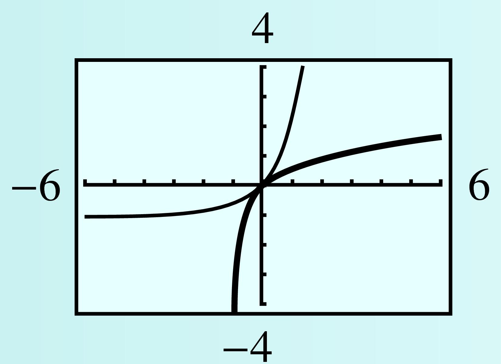
Checkpoint 5.59. Practice 10.
Find the inverse function for \(f(x) = 2 \log(x + 1)\text{.}\)
Graph \(f\) and \(f^{-1}\) in the window
\begin{equation*}
\begin{aligned}[t]
\text{Xmin} \amp = -6 \amp\amp \text{Xmax} = 6\\
\text{Ymin} \amp = -4 \amp\amp \text{Ymax} = 4
\end{aligned}
\end{equation*}
State the domain and range of \(f\) and \(f^{-1}\text{.}\)
Solution.
\(\displaystyle f^{-1}(x) = 10^{x/2} - 1 \)
Domain of \(f\text{:}\) \((-1,\infty)\text{;}\) Range of \(f\text{:}\) all real numbers; Domain of \(f^{-1}\text{:}\) all real numbers; Range of \(f^{-1}\text{:}\) \((-1, \infty)\)
Checkpoint 5.60. Pause and Reflect.
Compare the graphs of \(f(x)=\log \dfrac{1}{x}\) and \(g(x)=-\log x\text{,}\) and explain.